Differences between revisions 20 and 21
| Deletions are marked like this. | Additions are marked like this. |
| Line 94: | Line 94: |
| == Kepler Sage Analysis == | |
| Line 95: | Line 96: |
|
The data can also be analyzed by putting a wrapper around Kepler's algorithm. |
The data can also be analyzed by putting a wrapper around Kepler's algorithm, as described in. |
| Line 101: | Line 100: |
|
Using the code referenced above (sage_analysis_code.r), for a data matrix containing transcripts per million |
|
| Line 102: | Line 103: |
| # for data matrix mgex | |
| Line 129: | Line 131: |
|
attachment:solexa_RS2.jpg |
Using R to evaluate DGE for differential expression
Moderated statistical tests for assessing differences in tag abundance. (2007). Robinson MD, Smyth GK. Bioinformatics. 23(21):2881-7. PMID: 17881408
The authors of this paper develop a statistical test using a negative binomial distribution to model noise in the data. They release R code (available at bioinf.wehi.edu.au/resources/) to support their treatment, but it is uncommented. The windows version installs from their zip file, but I was unable to get the linux version to build.
Here I apply the code and examine the results in a sample data set.
At the website above you can find a tar archive called: msage_0.7.tar.gz. I can't get the package to install in R, so I simply unpack it and use the .R files directly. In addition, the code calls a code block (kepler.R) which is not included in the distribution. However, it is available here: http://dulci.biostat.duke.edu/sage/sage_analysis_code.r
Incidentally, the block of code: kepler.R is not actually required for the Robinson-Smyth algorithm. It is only called for the comparison of their algorithm to Kepler's algorithm quoted in the paper.
Basically there are two files of R code in the msage package: fitNBP.R and msage.R that can be sourced. The file msage.R has a source statement inside: source("kepler.R"), however this code block is not included. To get the code to function, download sage_analysis.r, and rename it kepler.R (written by Thomas Kepler at Duke). It contains a function called: glm.poisson.disp() that is called by msage.R.
Since I can't get the package to install, I simply place the .R files in my working directory (along with kepler.R), and source them:
# set working directory and load library functions
setwd("E:/cry1/Solexa/Smyth")
source("fitNBP.R")
source("msage.R")
This doesn't strike me as the optimal way to proceed, as you end up with a messy workspace (71 items in your environment), but I don't know a better way.
Assemble some data
There is a function in msage which can assemble data from individual tab-delimited tag files of the form: tag, count. It's called: read.sage() and takes an array of file names to read. It returns a list with two elements: a data matrix in the first position, and an array of library sizes as the second element. The input files simply need two columns, lists of tags (or gene names) and the associated counts separated by a tab character. They do not have to be normalized to tpm.
Assuming you had a directory of tag results files you could read them in as follows:
# read mydir to get a list of file names with .txt extensions
files <- dir("mydir", "txt", full.n=T)
# read in files of my choosing
dge <- read.sage(files[c(3,4,7,8)])
dge will now be a list containing a data matrix with counts for all the tags from all the files that were read, and an array with the total counts found in each file (also known as the size of each library).
However I already have my data in a table.
                wt1     wt2     mut1    mut2
NM_008665       3347    2740    3185    2842
CF805324        3336    2897    3500    2838
NM_030248       3252    2754    3231    2604
BC093504        3241    3179    3482    2943
AK043166        3157    7257    55      8837
NM_133703       3153    3196    2839    3588
NM_198419       3131    2787    2631    3576
BX511437        2893    2017    2429    2059
NM_028110       2844    2611    2279    2237
BF470700        2830    2629    3343    2333
AK028146        2681    2464    2104    2501
...
Once we have some data we need to make a list to hand to the first function. The list contains the data matrix, the sample groupings, and the library sizes. You may want to filter your data to only contain rows of the matrix that have reasonable tag counts. A set of columns with only 1 count in half of them won't be very meaningful.
My data is in a table called gex.all (if it's a data frame you can reference it as.matrix as I do below). I need to find the size of each library (aka the sum of each column), and I want to filter it a little:
lib.size <- colSums(gex.all)
# create a filter for really low numbers of reads
k <- rowSums(gex.all) > 4

# create a list structure
cws <- list(data=as.matrix(gex.all[k,]), groups=c(1,1,2,2), lib.size=lib.size)

# run the first function from msage
# this takes a while
alpha <- alpha.approxeb(cws)

# this takes a while
ms <- msage(cws, alpha=alpha$alpha)

adj.p <- p.adjust(ms$exact, "fdr")
k <- (adj.p < .05)

# create table with some results
all <- cbind(cws$data,adj.p,sign(rowSums(cws$data[,1:2]) - rowSums(cws$data[,3:4])))

# save results to disk
write.table(all[k,], "all.csv", sep=",", col.names=NA)
The functions: alpha.approxeb() and msage() took a combined time of 36 hours to run on a data set with 18000 rows.
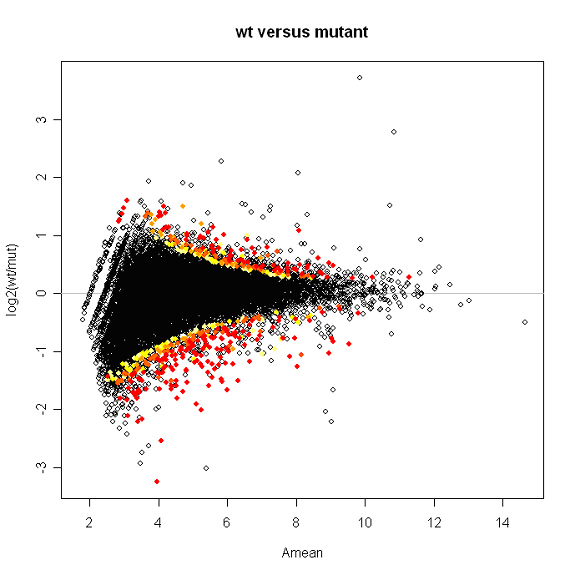
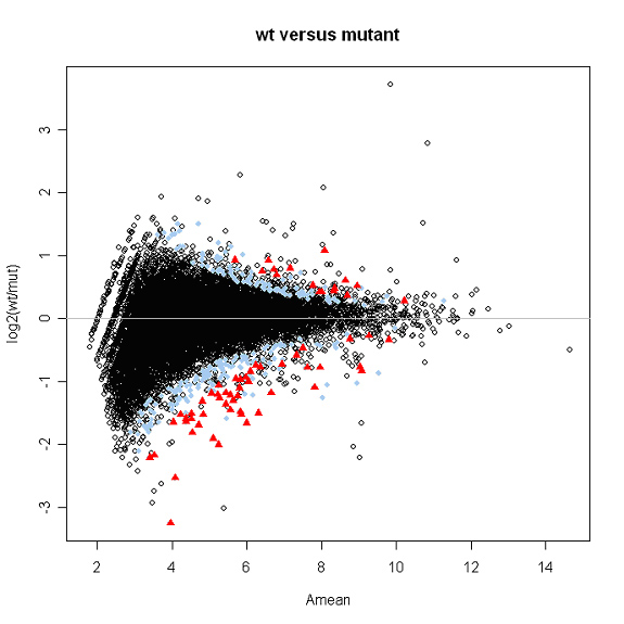
Plotted below is a snapshot of the results. Spots are labeled with a color gradient based on p-value. Red spots have p-values of 0.01 or less.

Kepler Sage Analysis
The data can also be analyzed by putting a wrapper around Kepler's algorithm, as described in.
Identifying differential expression in multiple SAGE libraries: an overdispersed log-linear model approach. (2005). Lu J, Tomfohr JK, Kepler TB. BMC Bioinformatics. 6:165. PMID: 15987513
Using the code referenced above (sage_analysis_code.r), for a data matrix containing transcripts per million
# for data matrix mgex
results <- c()
for(i in 1:nrow(mgex)){
  tag.count <- as.numeric(mgex[i,])

  #fit the overdispersed log-linear model
  fit <- glm(tag.count~offset(log(lib.size))+group,family=poisson(link=log));
  fit.ps <- glm.poisson.disp(fit,verbose=FALSE);
  phi <- fit.ps$dispersion;
  t.value <- summary(fit.ps)$coefficients[2,'z value'];
  p.value <- 2*pt(-abs(t.value),fit.ps$df.residual);

  results <- rbind(results, c(tag.count, t.value, phi, p.value))

  # spit out some output so I know things are happening
  if( ! i %% 100 ){
     cat("row number ", i, "\n")
     flush.console()
  }
}

rownames(results) <- rownames(mgex)
colnames(results) <- c(colnames(mgex), "t", "phi", "p")

write.table(results, file="kepler_sage_results.txt", sep=",", col.names=NA)

CategoryR ChrisSeidel
